
Simulating oil distribution inside a spinning e-motor takes seconds. Predicting how component temperatures evolve under real operating loads takes minutes. Those two timescales belong to different physical problems, and no single simulation method bridges them economically. The engineers who get EDU thermal predictions right are not simply running one tool longer, they are connecting two methods intelligently. And the cost of not doing that shows up not only in compute bills, but in missed hotspots and incorrect insulation class selections.
Intro
If you work on EDU cooling, you have likely run into this problem. This article walks through why the timescale gap exists, where conventional approaches break down, and how to couple particle CFD with a 3D/1D hybrid thermal model in a way that delivers spatially resolved hotspot predictions at design-iteration speed. The workflow and numbers referenced come from our EDU case study with shonDy and shonTA.
Why Timescale Mismatch Matters
Winding insulation degrades with temperature. As a widely used engineering rule of thumb, every 10°C increase in sustained operating temperature roughly halves insulation service life. This rule of thumb is an approximation of the Arrhenius-type thermal aging described in the IEC 60085 framework. In practice, the actual halving interval is material-specific and has to be determined for each material individually.
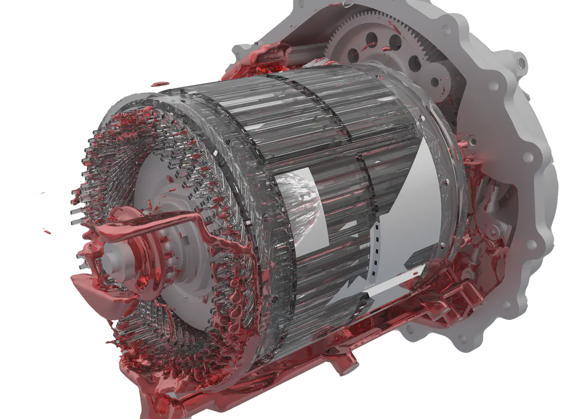
Two simulation problems sit at the core of that design question. The first is fluid: where does the oil go inside the machine, and which surfaces are actually wetted across different operating points? This is a free-surface problem that stabilises within seconds. The second is thermal: how do component temperatures evolve as heat accumulates over the drive cycle? This unfolds over minutes. The physics are different, the timescales are different, and no single simulation method handles both efficiently.
The Boundary Condition Problem
The standard workaround is to decouple the two analyses: run a physical short CFD simulation for oil distribution, then set thermal boundary conditions manually using empirical heat transfer coefficient (HTC) correlations before running the thermal model. This works in simple geometries. In an EDU it introduces errors that compound.
Empirical HTC correlations are calibrated for uniform flow over simplified surfaces like tubes, flat plates, and annular gaps. Inside a spinning e-motor, the oil distribution is geometry-dependent and strongly asymmetric. The end winding on the shaft side may receive direct oil jet contact, while the far end sees only a splash. Static baffles, shaft channels, and rotor geometry all influence where oil ends up. A single average HTC applied across the entire winding surface smooths over exactly the variation that determines hotspot location.
The risk: a thermal model built on averaged or empirical HTCs may predict a safe peak winding temperature while the actual hotspot, in the region that receives least oil contact, sits significantly higher. In a pure Lumped Parameter Thermal Network (LPTN), each component is represented as a single temperature node, meaning the winding has one temperature value, not a distribution. That single value can look safe while a localised hotspot within that same component is critically high. That difference does not show up until testing, or worse, in the field.
The alternative, running particle CFD for the full duration of a drive cycle, is impractical. Particle methods carry a computational cost that scales steeply with simulated time at the resolutions needed to resolve oil films on winding surfaces. Minutes of physical time would require weeks of computing.
The Coupling Method
The practical solution is to use the short particle CFD simulation for what it is actually good at: characterising the quasi-stationary oil distribution and extracting spatially resolved HTCs, then handing that data off as boundary conditions to a fast thermal model that handles the slow dynamics.
This works because oil distribution in an EDU reaches quasi-steady state within seconds at a given operating point. The HTC field on the winding and stator surfaces stabilises before component temperatures have had time to change meaningfully. The short simulation is genuinely representative of the thermal boundary conditions during sustained operation.
The output of the particle CFD step is not a single average HTC per surface, it is a spatially resolved point cloud that tells the thermal model that one side of the winding sees direct oil contact while the other sees little to no coverage. That distribution, mapped onto the nodes of the 3D/1D hybrid thermal model, is what separates a hotspot prediction from a temperature estimate. Unlike a pure LPTN, the hybrid approach resolves heat development within each component using 3D FEM, meaning the spatially resolved HTCs from the particle CFD step feed into a model that can actually show where inside the winding the temperature peaks.
Setup Checklist: What the Coupling Workflow Requires
The methodology is straightforward to follow, but specific setup choices determine whether the HTC handoff is reliable. The following reflects what the workflow requires at each stage.
Particle CFD stage
- Include all rotating components at target RPM, oil distribution is centrifuge-driven and speed-dependent
- Use realistic oil volume and shaft inlet flow rate, these set the wetted area directly
- Run until HTC values on the winding and stator surfaces stabilise
- Extract HTC as a spatially resolved output, not a per-component average
- Repeat at 2-3 representative operating points if drive cycle interpolation is needed
Thermal model stage
- Map the HTC point cloud to corresponding LPTN convection nodes, not a single average per component
- Include thermal contact conductance between solids (shaft-rotor, rotor-magnets)
- Model shaft oil channels with a 1D flow network, where needed
- Run the thermal simulation over the full operating duration, the thermal model handles slow dynamics efficiently
- Check peak winding temperature against insulation class rating, not just average winding temperature
Results from our Case Study
In a concrete case(2,000 RPM motor speed, 1.6 L oil, 12 L/min shaft flow rate, 9 kW total thermal losses), HTC values on the winding and stator surfaces reached steady state at around 4.5 seconds into the particle CFD simulation. The spatial averages extracted were 160 W/m²K on the winding and 200 W/m²K on the stator. Those values are not uniform: the resolved distribution shows meaningfully higher HTCs in regions of direct oil contact.
Table 1: Key Results from the Coupled Simulation
| Metric | Value |
|---|---|
| HTC stabilisation time in particle CFD | ~4.5 s |
| Avg. winding HTC | 160 W/m²K |
| Avg. stator HTC | 200 W/m²K |
| Peak winding temperature predicted | 235 °C |
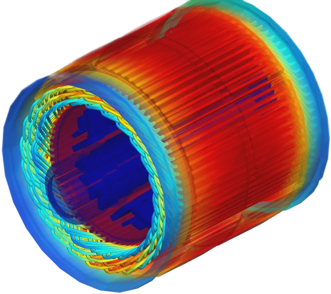
Fed into the 3D/1D hybrid thermal model, the coupled simulation predicted a system temperature range of 80°C (initial oil temperature) to 235°C at peak winding temperature. The heat path is clearly resolved: energy flows from the windings into the stator and is released to the environment. The 235°C peak is the number that drives insulation class selection, and it is only accessible because the thermal model received a spatially resolved HTC distribution rather than a bulk average.
Table 2: Comparison of Thermal Boundary Condition Approaches. Particle CFD to Thermal Network coupling combines hotspot-resolution accuracy with drive-cycle simulation efficiency, bridging the gap between empirical thermal networks and full 3D CFD.
| Approach | HTC Input | Hotspot Accuracy | Drive Cycle Speed |
|---|---|---|---|
| LPTN with empirical correlations | Single average per surface | Misses asymmetric hotspots | Fast |
| Full 3D CFD + thermal | Fully resolved | High | Impractical for drive cycles |
| Particle CFD → Network | Spatially resolved per region | High (hotspot location captured) | Practical for design iteration |
Conclusion
The timescale gap in EDU thermal simulation is a real engineering constraint, not a software limitation. Particle CFD and the 3D/1D hybrid thermal model are not competing methods but complementary ones, each suited to a specific part of the problem. The particle simulation gives you the oil distribution and surface HTCs that the thermal model cannot generate on its own. The 3D/1D hybrid thermal model gives you the temperature evolution over time, with 3D FEM resolving heat development inside each component, at a cost that the particle simulation cannot sustain economically. Connected correctly, with spatially resolved HTCs as the handoff point, the combined workflow delivers hotspot predictions that are accurate enough to drive insulation class decisions and cooling circuit design, at a speed that fits the design iteration phase, not just final validation.
If you are working on EDU cooling and want to apply this workflow to your own design, request a trial on shonDy and shonTA.