In computational fluid dynamics (CFD), spatial discretization, specifically the process of mesh generation and partitioning, plays a critical role in determining the accuracy and efficiency of numerical simulations. The mesh defines how the continuous physical domain is subdivided into discrete control volumes, over which the governing equations are solved. Broadly, engineering applications employ two primary mesh types: structured and unstructured meshes.
A structured mesh is characterized by a regular grid topology, where each internal node has a consistent number and arrangement of neighbouring cells, typically forming hexahedral elements. This uniform structure facilitates an implicit definition of node connectivity based on mesh indices, eliminating the need for explicit neighbour storage. Structured meshes generally yield higher numerical accuracy and better convergence behaviour due to their superior element quality and smooth variation of grid spacing. However, generating structured meshes for complex geometries is often labour-intensive, requiring significant manual intervention and, in many cases, simplification of the original geometry to achieve a topologically regular grid.
In contrast, an unstructured mesh lacks this regular connectivity pattern. Internal nodes may have varying numbers of adjacent elements, which can take on diverse shapes such as tetrahedra, prisms, pyramids, or general polyhedra. The flexibility of unstructured meshes enables automated mesh generation for geometrically complex domains, making them suitable for simulations involving intricate boundaries or multiple interacting components. Nevertheless, this flexibility comes at the cost of increased memory requirements and computational overhead, as neighbour relationships must be explicitly stored and accessed during numerical calculations.
Octree Meshes
The octree, as a method for organising spatial objects, divides space into cells based on unit density, thereby avoiding the need to iterate over all objects during mesh generation. Its principle is relatively straightforward: when the partitioning conditions are met, the three-dimensional space is divided into eight equal sections, with spatial objects allocated accordingly. An octree mesh, a common form of unstructured mesh, is generated by first partitioning the computational domain into one or more large cubic meshes. These large cubic meshes are then recursively subdivided into eight sub-meshes until each sub-mesh meets predefined size requirements or is clipped by geometric boundaries.
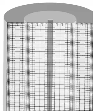
Although octrees are unstructured meshes, their internal hexahedra of varying sizes maintain fixed refinement relationships. This allows indirect storage of mesh cell geometry and neighbour relationships during mesh storage. Here, we introduce a method that utilises the Space-Filling Curve (SFC) to store mesh cells.
Space-Filling Curves (SFC)
A space-filling curve is a one-dimensional interval that contains a mapping from n-dimensional space to one-dimensional space. Conceptually, it can be viewed as a continuous path that visits every discrete point within a spatial domain in a specific order. This order may inherently possess certain spatial positional characteristics, thereby facilitating cache layout optimisation.
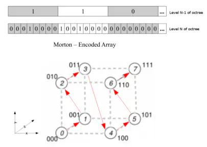
The Morton curve, a common space-filling curve, maps n-dimensional space to a sorted linear sequence. When applied to coordinates, the Morton code defines a Z-shaped space-filling curve, hence known as the Z-curve. This encoding ensures that points close in physical space tend to have similar Morton codes, a property that greatly benefits memory layout and parallel data access.
2.1 Generation of Morton Codes
The generation of Morton codes essentially involves bit interleaving of the given coordinates across each dimension.
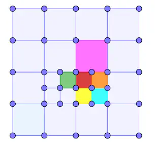
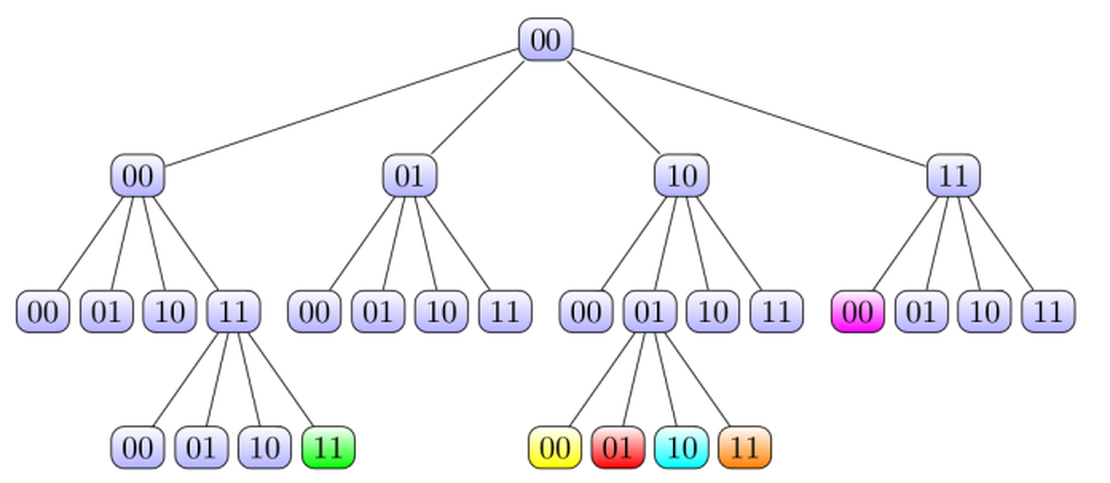
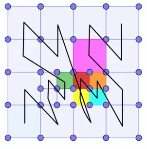
For illustrative purposes, consider a quadtree grid in a two-dimensional plane with a maximum refinement level of maxLevel = 2. The root node of the tree represents the grid’s bounding box, while leaf nodes correspond to individual grid cells. Each cell is assigned a six-bit binary code, typically based on the cell’s centroid position. The total number of bits in the Morton code is:
where numDim denotes the spatial dimension of the grid and maxLevel represents the maximum refinement level.
The bit code for each quadtree cell can be specified by its relative index within the Cartesian coordinate system. For instance, the Morton code for the red cell in Figure 3 may be denoted as (10,01,01). The grid boundary 00, representing the initial coarsest grid, is excluded from the Morton code. The binary Morton code may be converted to decimal when required; for instance, the decimal sequence number for the red cell is 37. All cells of this quadtree grid can be arranged into a tree as shown in Figure 4, where the coloured cells correspond to the two-dimensional quadtree cells in Figure 3.
Once all cell Morton codes are generated, traversing from the bottom-left cell to the top-right cell yields the spatial traversal sequence depicted by the black curve in Figure 5. This curve exhibits a distinct zigzag structure; hence, the Morton curve is also known as the Z-curve. It is observed that sibling cells within the quadtree also occupy adjacent positions along the Morton curve. Furthermore, during dynamic refinement of the quadtree, newly generated sibling cells cluster within the vicinity of their parent cell’s position on the Morton curve. When refining octrees in three-dimensional space, the Morton codes of octree cells exhibit analogous spatial characteristics.
2.2 Number of Refinement Levels
Once the Morton code is generated, the refinement level of each cell can be directly deduced from the Morton code.
For a Morton code of dimension dim, the algorithm is as follows: given a Morton code as an array of length N, mortonKey, and an octree/quadtree mesh, which is a collection of Morton codes.

For instance, the pink cell in Figure 3 has a Morton code of (11, 00, 00). Initially set level = N/dim = 3. Starting from the first layer of the Morton code, code 11 (non-zero) skips to the next layer. The second layer’s Morton code is 00; flipping the x-bit of 00 yields 10. Checking (11, 10, 00) reveals it already exists in the quadtree, indicating the presence of sibling neighbours at level 2. Proceeding to the third layer, the Morton code is 00. Flipping the x-bit of 00 yields 10. Checking reveals that (11, 00, 10) does not exist in the quadtree. Thus, level = level - 1 = 2. Consequently, this cell has two refinement levels.
2.3 Cell Geometric Information
From the Morton code and the geometric centre and edge length of the root node cell, the edge length, geometric centre, and vertex positions of the refined cells can be obtained.
2.4 Neighbour Information of Cells
The significance of cell neighbour information for PDE numerical computation is self-evident. The storage and retrieval of neighbour information substantially impact the overall computational efficiency of PDE solvers. For quadtree/octree cells employing Morton codes, neighbour information is inherently embedded within the Morton code, accessible through straightforward bitwise operations.
Neighbours of quadtree/octree cells are categorised as sibling neighbours and non-sibling neighbours. Sibling neighbours indicate adjacent cells sharing a common parent cell with the current cell. Non-sibling neighbours denote cells with no sibling relationship to the current cell.
2.4.1 Peer Neighbours
For instance, the sibling neighbours of the red cell (10,01,01) include the yellow cell (10,01,00) and the orange cell (10,01,11). The first four binary digits (10,01) of the Morton codes for these three cells are identical, indicating they are sibling cells. The fifth binary digit of the red cell, 0, represents the x-direction, while the sixth bit’s 1 denotes the y-direction. To locate neighbours along the x-direction, one needs to only preserve the fifth and sixth binary digits and invert the 0 to obtain a 1, thereby finding the x-aligned sibling neighbour (10,01,11), namely the orange cell.
To locate the non-sibling neighbour of the red cell, the green cell (00,11,11), bit operations can be performed in both directions. For instance, determining the non-sibling neighbour along the x-axis for the red cell (10,01,01) proceeds as follows:
Identify the bit-flip layer position along a specific axis. The Morton code of this cell at the highest refinement layer is 01, meaning the binary bit in the x-direction is 0. Tracing upwards to its parent layer, the binary code is 01, where the x-direction binary bit remains 0. Tracing further upwards to the grandparent layer, the binary number is 01, where the x-direction binary bit changes to 1. Thus, this layer is the bit-flipping layer. That is, from left to right, the binary bit in the x-direction is (1,0,0), and the first layer is the bit-flipping layer.
Flip the binary bit at the corresponding bit-flipping layer. For the red cell (10,01,01), its bit-flipping layer in the x-direction has been determined to be the first layer. To determine the non-sibling neighbour of the red cell, we invert the Morton code of the red cell in the x-direction (1,0,0) up to the first layer, yielding (0,1,1). The Morton code in the y-direction (0,1,1) remains unchanged, yielding (00,11,11), which corresponds precisely to the green cell.
2.4.2 Cross-Level Neighbours
To determine neighbours with differing refinement levels in a given direction, the following method is employed, taking the pink cell (11,00,00)’s non-sibling neighbour in the y-direction as an example:
Similar to Section 2.4.1, the pink cell’s Morton code is (11,00,00), confirming the bit-reversal layer as the second layer. Thus, reversing the y-axis Morton code (1,0) yields (0,1), while the x-axis remains unchanged, resulting in the Morton code (10,01).
The refinement level of the cell at (10,01) is higher than the current pink cell. Therefore, the last two digits must be repeated at the third layer to yield (10, 01, 01), which corresponds to the red cell. The red cell is one of the pink cell’s cross-level neighbours. To locate its other neighbour, one needs to only find the red cell’s x-axis sibling neighbour. This is obtained by flipping the x-axis bit in 01, yielding the orange cell (10, 01, 11).
Thus, both y-axis cross-level neighbours (10,01,11) and (10,01,01) of the pink cell are fully determined.
Advantages of Morton Coding
Data Compression: The construction method of Morton code is relatively straightforward, converting coordinate values representing multidimensional data into a single integer. Various geometric and topological information about grid cells can be readily obtained from bitwise operations on the Morton code, significantly reducing the size of the data stored and transmitted.
Data Locality: Following Morton code sorting, adjacent grid cells frequently correspond to physically contiguous locations. This enhances cache hit rates and memory bandwidth, thereby better leveraging modern processors’ parallel computing capabilities to execute more complex computational tasks.
Computational Efficiency: Morton code sorting substantially reduces redundant computations, consequently improving computational speed and overall efficiency.